Property Specification
In this section we present how to specify protocol properties
as trace and observational equivalence properties, based on the
action facts given in the model. Trace properties are given as
guarded first-order logic formulas and observational equivalence
properties are specified using the diff operator,
both of which we will see in detail below.
Trace Properties
The Tamarin multiset rewriting rules define a labeled transition system. The system’s state is a multiset (bag) of facts and the initial system state is the empty multiset. The rules define how the system can make a transition to a new state. The types of facts and their use are described in Section Rules. Here we focus on the action facts, which are used to reason about a protocol’s behaviour.
A rule can be applied to a state if it can be instantiated such that its left hand side is contained in the current state. In this case, the left-hand side facts are removed from the state, and replaced by the instantiated right hand side. The application of the rule is recorded in the trace by appending the instantiated action facts to the trace.
For instance, consider the following fictitious rule
rule fictitious:
   [ Pre(x), Fr(~n) ]
 --[ Act1(~n), Act2(x) ]-->
   [ Out(<x,~n>) ]
The rule rewrites the system state by consuming the facts
Pre(x) and Fr(~n) and producing the fact
Out(<x,~n>). The rule is labeled with the
actions Act1(~n) and Act2(x). The rule
can be applied if there are two facts Pre and
Fr in the system state whose arguments are matched by
the variables x and ~n. In the
application of this rule, ~n and x are
instantiated with the matched values and the state transition is
labeled with the instantiations of Act1(~n) and
Act2(x). The two instantiations are considered to
have occurred at the same timepoint.
A trace property is a set of traces. We define a set of traces in Tamarin using first-order logic formulas over action facts and timepoints. More precisely, Tamarin’s property specification language is a guarded fragment of a many-sorted first-order logic with a sort for timepoints. This logic supports quantification over both messages and timepoints.
The syntax for specifying security properties is defined as follows:
Allfor universal quantification, temporal variables are prefixed with #Exfor existential quantification, temporal variables are prefixed with #==>for implication&for conjunction|for disjunctionnotfor negationf @ ifor action constraints, the sort prefix for the temporal variable ‘i’ is optionali < jfor temporal ordering, the sort prefix for the temporal variables ‘i’ and ‘j’ is optional#i = #jfor an equality between temporal variables ‘i’ and ‘j’x = yfor an equality between message variables ‘x’ and ‘y’Pred(t1,..,tn)as syntactic sugar for instantiating a predicate Pred for the termst1totn
All action fact symbols may be used in formulas. The terms (as arguments of those action facts) are more limited. Terms are only allowed to be built from quantified variables, public constants (names delimited using single-quotes), and free function symbols including pairing. This excludes function symbols that appear in any of the equations. Moreover, all variables must be guarded. If they are not guarded, Tamarin will produce an error.
Predicates
Predicates are defined using the predicates
construct, and substituted while parsing trace properties, whether
they are part of lemmas, restrictions or embedded
restrictions:
builtins: multiset
predicates: Smaller(x,y) <=> Ex z. x + z = y

[..]

lemma one_smaller_two:
    "All x y #i. B(x,y)@i ==> Smaller(x,y)"
Guardedness
To ensure guardedness, for universally quantified variables, one has to check that they all occur in an action constraint right after the quantifier and that the outermost logical operator inside the quantifier is an implication. For existentially quantified variables, one has to check that they all occur in an action constraint right after the quantifier and that the outermost logical operator inside the quantifier is a conjunction. We do recommend to use parentheses, when in doubt about the precedence of logical connectives, but we follow the standard precedence. Negation binds tightest, then conjunction, then disjunction and then implication.
To specify a property about a protocol to be verified, we use
the keyword lemma followed by a name for the property
and a guarded first-order formula. This expresses that the
property must hold for all traces of the protocol. For instance,
to express the property that the fresh value ~n is
distinct in all applications of the fictitious rule (or rather, if
an action with the same fresh value appears twice, it actually is
the same instance, identified by the timepoint), we write
lemma distinct_nonces:
    "All n #i #j. Act1(n)@i & Act1(n)@j ==> #i=#j"
or equivalently
lemma distinct_nonces:
  all-traces
    "All n #i #j. Act1(n)@i & Act1(n)@j ==> #i=#j"
We can also express that there exists a trace for which the
property holds. We do this by adding the keyword
exists-trace after the name and before the property.
For instance, the following lemma is true if and only if the
preceding lemma is false:
lemma distinct_nonces:
  exists-trace
    "not All n #i #j. Act1(n)@i & Act1(n)@j ==> #i=#j"
Secrecy
In this section we briefly explain how you can express standard secrecy properties in Tamarin and give a short example. See Protocol and Standard Security Property Specification Templates for an in-depth discussion.
Tamarin’s built-in message deduction rule
rule isend:
   [ !KU(x) ]
 --[  K(x)  ]-->
   [ In(x)  ]
allows us to reason about the Dolev-Yao adversary’s knowledge.
To specify the property that a message x is secret,
we propose to label a suitable protocol rule with a
Secret action. We then specify a secrecy lemma that
states whenever the Secret(x) action occurs at
timepoint i, the adversary does not know
x.
lemma secrecy:
  "All x #i.
    Secret(x) @i ==> not (Ex #j. K(x)@j)"
Example. The following Tamarin theory
specifies a simple one-message protocol. Agent A
sends a message encrypted with agent B’s public key
to B. Both agents claim secrecy of a message, but
only agent A’s claim is true. To distinguish between
the two claims we add the action facts Role('A')
(respectively Role('B')) to the rule modeling role
A (respectively to the rule for role B).
We then specify two secrecy lemmas, one for each role.
theory secrecy_asym_enc
begin

builtins: asymmetric-encryption

/* We formalize the following protocol:

    1. A -> B: {A,na}pk(B)

*/

// Public key infrastructure
rule Register_pk:
  [ Fr(~ltkX) ]
  -->
  [ !Ltk($X, ~ltkX)
  , !Pk($X, pk(~ltkX))
  , Out(pk(~ltkX))
  ]

// Compromising an agent's long-term key
rule Reveal_ltk:
  [ !Ltk($X, ltkX) ] --[ Reveal($X) ]-> [ Out(ltkX) ]

// Role A sends first message
rule A_1_send:
  [ Fr(~na)
  , !Ltk($A, ltkA)
  , !Pk($B, pkB)
  ]
--[ Send($A, aenc(<$A, ~na>, pkB))
  , Secret(~na), Honest($A), Honest($B), Role('A')
  ]->
  [ St_A_1($A, ltkA, pkB, $B, ~na)
  , Out(aenc(<$A, ~na>, pkB))
  ]

// Role B receives first message
rule B_1_receive:
  [ !Ltk($B, ltkB)
  , In(aenc(<$A, na>,pk(ltkB)))
  ]
--[ Recv($B, aenc(<$A, na>, pk(ltkB)))
  , Secret(na), Honest($B), Honest($A), Role('B')
  ]->
  [ St_B_1($B, ltkB, $A, na)
  ]

lemma executable:
  exists-trace
    "Ex A B m #i #j. Send(A,m)@i & Recv(B,m) @j"

lemma secret_A:
  all-traces
    "All n #i. Secret(n) @i & Role('A') @i ==> (not (Ex #j. K(n)@j)) | (Ex B #j. Reveal(B)@j & Honest(B)@i)"

lemma secret_B:
  all-traces
    "All n #i. Secret(n) @i & Role('B') @i ==> (not (Ex #j. K(n)@j)) | (Ex B #j. Reveal(B)@j & Honest(B)@i)"


end
In the above example the lemma secret_A holds as
the initiator generated the fresh value, while the responder has
no guarantees, i.e., lemma secret_B yields an
attack.
Authentication
In this section we show how to specify a simple message authentication property. For specifications of the properties in Lowe’s hierarchy of authentication specifications (Lowe 1997) see the Section Protocol and Standard Security Property Specification Templates.
We specify the following message authentication
property: If an agent a believes that a message
m was sent by an agent b, then
m was indeed sent by b. To specify
a’s belief we label an appropriate rule in
a’s role specification with the action
Authentic(b,m). The following lemma defines the set
of traces that satisfy the message authentication property.
lemma message_authentication:
    "All b m #j. Authentic(b,m) @j ==> Ex #i. Send(b,m) @i &i<j"
A simple message authentication example is the following
one-message protocol. Agent A sends a signed message
to agent B. We model the signature using asymmetric
encryption. A better model is shown in the section on
Restrictions.
theory auth_signing_simple
begin

builtins: asymmetric-encryption

/* We formalize the following protocol:

    1. A -> B: {A,na}sk(A)

*/

// Public key infrastructure
rule Register_pk:
  [ Fr(~ltkX) ]
  -->
  [ !Ltk($X, ~ltkX)
  , !Pk($X, pk(~ltkX))
  , Out(pk(~ltkX))
  ]

// Role A sends first message
rule A_1_send:
  [ Fr(~na)
  , !Ltk($A, ltkA)
  ]
--[ Send($A, <$A, ~na>)
  ]->
  [ St_A_1($A, ltkA, ~na)
  , Out(aenc(<$A, ~na>,ltkA))
  ]

// Role B receives first message
rule B_1_receive:
  [ !Pk($A, pk(skA))
  , In(aenc(<$A, na>,skA))
  ]
--[ Recv($B, <$A, na>)
  , Authentic($A,<$A, na>), Honest($B), Honest($A)
  ]->
  [ St_B_1($B, pk(skA), $A, <$A, na>)
  ]

lemma executable:
  exists-trace
    "Ex A B m #i #j. Send(A,m)@i & Recv(B,m) @j"

lemma message_authentication:
    "All b m #i. Authentic(b,m) @i
     ==> (Ex #j. Send(b,m) @j & j<i)"

end
Property Development in the GUI
It is often just as hard to come up with the correct properties for a model than it is come up with the correct model for a protocol. Sometimes, you phrased the property too strong and there are trivial attacks you meant to exclude. Sometimes, you simply make mistakes.
Tamarin allows you to edit, add, and delete the lemmas of a theory in the GUI without requiring you to restart the server. Especially for large theories, editing lemmas in the GUI can save you significant amounts of time.
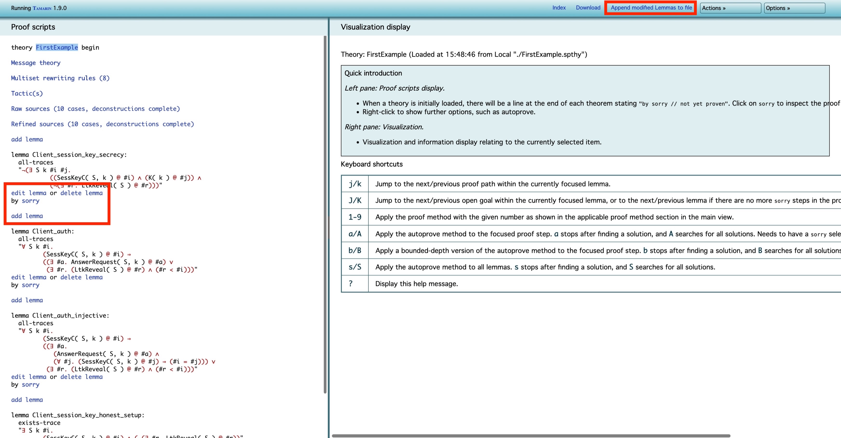
In the left half of your screen, you will find three buttons to add, delete, or edit lemmas. If you click any of these buttons, you will be shown more documentation, but their functionality should be self-explanatory for the most part. In general, the following applies when editing lemmas in the GUI:
- Your changes are not stored in your model file. If you want to persist your changes, you must either use “Download source” from the Actions menu to download the entire theory, or use “Append modified lemmas to file” from the Actions menu. This option will add new or modified lemmas at the end of your model file as a comment. You must then manually merge them into your model.
- Whenever you delete or edit a lemma marked as
reuse, all proofs after the deleted or edited lemma will be invalidated. This is because Tamarin cannot be certain anymore whether the proofs still hold. The proofs, though, will not be discarded, and you can again verify them. Tamarin will let you know should it encounter any issues. - You cannot add, modify, or delete sources lemmas. This is because sources lemmas influence Tamarin’s precomputations. You must edit sources lemmas in your model file and use “Reload file” from the Actions menu to reload the theory with the updated sources lemmas. If the theory was uploaded or modified interactively in the web interface, reloading is not possible, and you will have restart the server instead.
Below, we highlight the four most important buttons for editing lemmas in the GUI.
Observational Equivalence
All the previous properties are trace properties, i.e., properties that are defined on each trace independently. For example, the definition of secrecy required that there is no trace where the adversary could compute the secret without having corrupted the agent.
In contrast, Observational Equivalence properties reason about two systems (for example two instances of a protocol), by showing that an intruder cannot distinguish these two systems. This can be used to express privacy-type properties, or cryptographic indistinguishability properties.
For example, a simple definition of privacy for voting requires
that an adversary cannot distinguish two instances of a voting
protocol where two voters swap votes. That is, in the first
instance, voter A votes for candidate a
and voter B votes for b, and in the
second instance voter A votes for candidate
b and voter B votes for a.
If the intruder cannot tell both instances apart, he does not know
which voter votes for which candidate, even though he might learn
the result, i.e., that there is one vote for a and one for b.
Tamarin can prove such properties for two systems that only
differ in terms using the diff( , ) operator.
Consider the following toy example, where one creates a public
key, two fresh values ~a and ~b, and
publishes ~a. Then one encrypts either
~a or ~b (modeled using the
diff operator) and sends out the ciphertext:
// Generate a public key and output it
// Choose two fresh values and reveal one of it
// Encrypt either the first or the second fresh value
rule Example:
    [ Fr(~ltk)
    , Fr(~a)
    , Fr(~b) ]
  --[ Secret( ~b ) ]->
    [ Out( pk(~ltk) )
    , Out( ~a )
    , Out( aenc( diff(~a,~b), pk(~ltk) ) )
    ]
In this example, the intruder cannot compute ~b as
formalized by the following lemma:
lemma B_is_secret:
  " /* The intruder cannot know ~b: */
    All B #i. (
      /* ~b is claimed secret implies */
      Secret(B) @ #i ==>
      /* the adversary does not know '~b' */
      not( Ex #j. K(B) @ #j )
    )
However, he can know whether in the last message
~a or ~b was encrypted by simply taking
the output ~a, encrypting it with the public key and
comparing it to the published ciphertext. This is captured using
observational equivalence.
To see how this works, we need to start Tamarin in
observational equivalence mode by adding a --diff to
the command:
tamarin-prover interactive --diff ObservationalEquivalenceExample.spthyNow point your browser to http://localhost:3001. After clicking on the
theory ObservationalEquivalenceExample, you should
see the following.
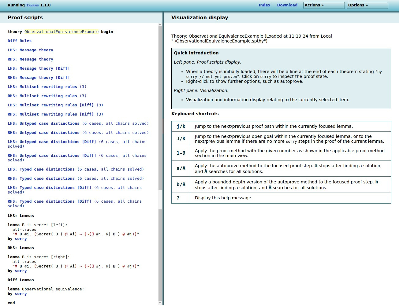
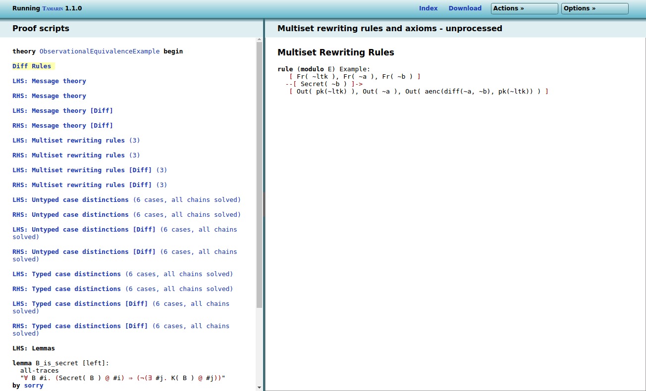
There are multiple differences to the ‘normal’ trace mode.
First, there is a new option Diff Rules, which
will simply present the rewrite rules from the .spthy
file. (See image below.)
Second, all the other points (Message Theory, Multiset Rewrite
Rules, Raw/Refined Sources) have been quadruplicated. The reason
for this is that any input file with the diff
operator actually specifies two models: one model where each
instance of diff(x,y) is replaced with x
(the left hand side, or LHS for short), and one model
where each instance of diff(x,y) is replaced with
y (the right hand side, or RHS for short).
Moreover, as the observational equivalence mode requires different
precomputations, each of the two models is treated twice. For
example, the point RHS: Raw sources [Diff] gives the
raw sources for the RHS interpretation of the model in
observational equivalence mode, whereas
LHS: Raw sources gives the raw sources for the LHS
interpretation of the model in the ‘trace’ mode.
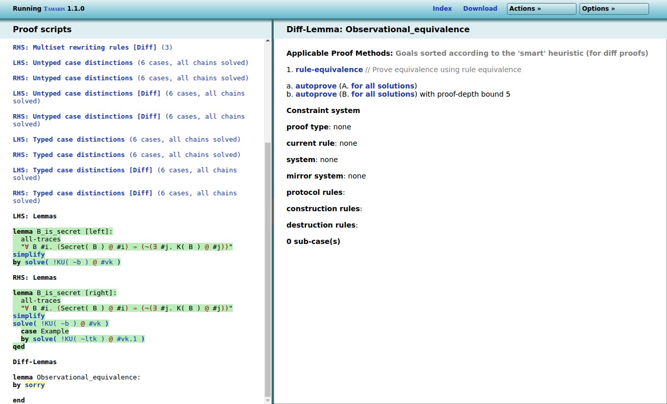
Third, all lemmas have been duplicated: the lemma
B_is_secret exists once on the left hand side (marked
using [left]) and once on the right hand side (marked
using [right]), as both models can differ and thus
the lemma needs to be proven on both sides.
Finally, there is a new lemma
Observational_equivalence, added automatically by
Tamarin (so no need to define it in the .spthy input
file). By proving this lemma we can prove observational
equivalence between the LHS and RHS models.
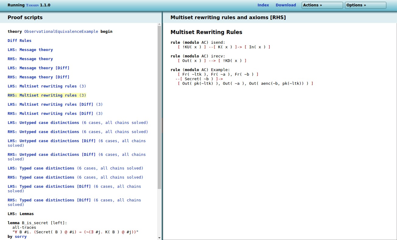
In the Diff Rules, we have the rules as written in
the input file:
If we click on LHS: Multiset rewriting rules, we
get the LHS interpretation of the rules (here
diff(~a, ~b) was replaced by ~a):
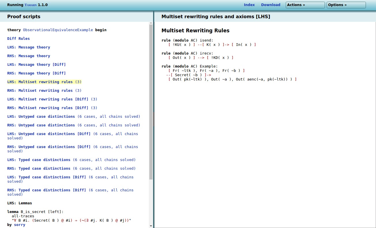
If we click on RHS: Multiset rewriting rules, we
get the RHS interpretation of the rules (here
diff(~a, ~b) was replaced by ~b):
We can easily prove the B_is_secret lemma on both
sides:
To start proving observational equivalence, we only have the
proof step 1. rule-equivalence. This generates
multiple subcases:
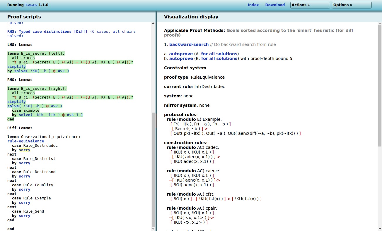
Essentially, there is a subcase per protocol rule, and there
are also cases for several adversary rules. The idea of the proof
is to show that whenever a rule can be executed on either the LHS
or RHS, it can also be executed on the other side. Thus, no matter
what the adversary does, he will always see ‘equivalent’
executions. To prove this, Tamarin computes for each rule all
possible executions on both sides, and verifies whether an
‘equivalent’ execution exists on the other side. If we continue
our proof by clicking on backward-search, Tamarin
generates two sub-cases, one for each side. For each side, Tamarin
will continue by constructing all possible executions of this
rule.
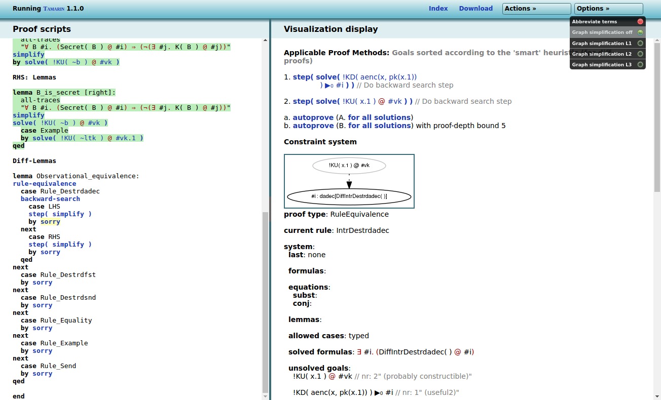
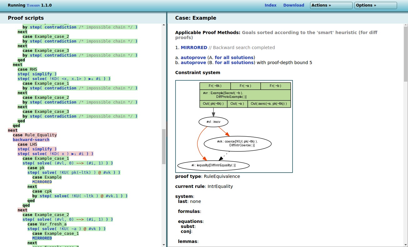
During this search, Tamarin can encounter executions that can be ‘mirrored’ on the other side, for example the following execution where the published key is successfully compared to itself:
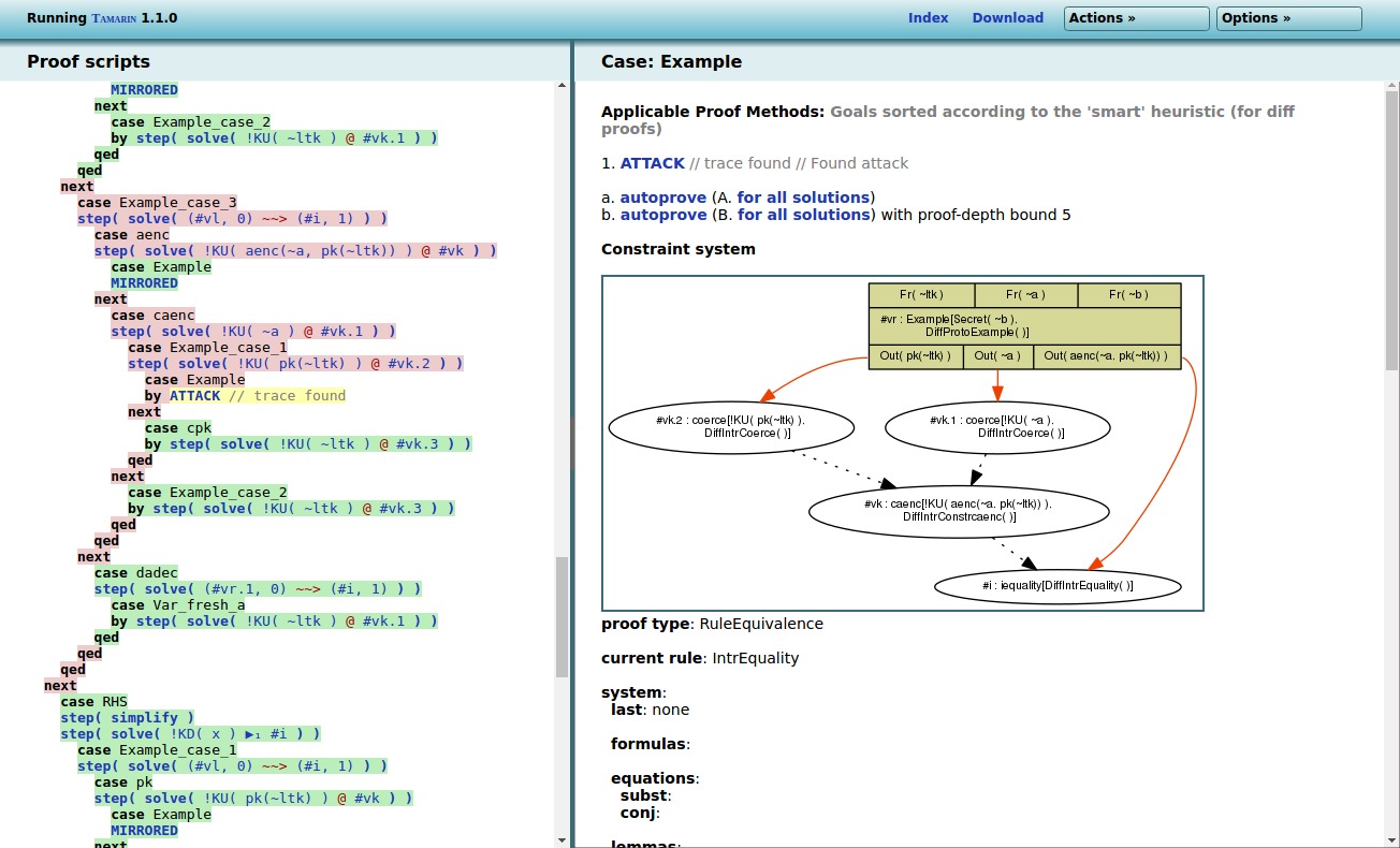
Or, Tamarin can encounter executions that do not map to the
other side. For example the following execution on the LHS that
encrypts ~a using the public key and successfully
compares the result to the published ciphertext, is not possible
on the RHS (as there the ciphertext contains ~b).
Such an execution corresponds to a potential attack, and thus
invalidates the “Observational_equivalence” lemma.
Note that Tamarin needs to potentially consider numerous possible executions, which can result in long proof times or even non-termination. If possible it tries not to resolve parts of the execution that are irrelevant, but this is not always sufficient.
Restrictions
Restrictions restrict the set of traces to be considered in the
protocol analysis. They can be used for purposes ranging from
modeling branching behavior of protocols to the verification of
signatures. We give a brief example of the latter. Consider the
simple message authentication protocol, where an agent
A sends a signed message to an agent B.
We use Tamarin’s built-in equational theory
for signing.
// Role A sends first message
rule A_1_send:
  let m = <A, ~na>
  in
  [ Fr(~na)
  , !Ltk(A, ltkA)
  , !Pk(B, pkB)
  ]
--[ Send(A, m)
  ]->
  [ St_A_1(A, ltkA, pkB, B, ~na)
  , Out(<m,sign(m,ltkA)>)
  ]

// Role B receives first message
rule B_1_receive:
  [ !Ltk(B, ltkB)
  , !Pk(A, pkA)
  , In(<m,sig>)
  ]
--[ Recv(B, m)
  , Eq(verify(sig,m,pkA),true)
  , Authentic(A,m), Honest(B), Honest(A)
  ]->
  [ St_B_1(B, ltkB, pkA, A, m)
  ]
In the above protocol, agent B verifies the
signature sig on the received message m.
We model this by considering only those traces of the protocol in
which the application of the verify function to the
received message equals the constant true. To this
end, we specify the equality restriction
restriction Equality:
  "All x y #i. Eq(x,y) @i ==> x = y"
The full protocol theory is given below.
theory auth_signing
begin

builtins: signing

/* We formalize the following protocol:

    1. A -> B: {A,na}sk(A)

using Tamarin's builtin signing and verification functions.

*/

// Public key infrastructure
rule Register_pk:
  [ Fr(~ltkA) ]
  -->
  [ !Ltk($A, ~ltkA)
  , !Pk($A, pk(~ltkA))
  , Out(pk(~ltkA))
  ]

// Compromising an agent's long-term key
rule Reveal_ltk:
  [ !Ltk(A, ltkA) ] --[ Reveal(A) ]-> [ Out(ltkA) ]

// Role A sends first message
rule A_1_send:
  let m = <A, ~na>
  in
  [ Fr(~na)
  , !Ltk(A, ltkA)
  , !Pk(B, pkB)
  ]
--[ Send(A, m)
  ]->
  [ St_A_1(A, ltkA, pkB, B, ~na)
  , Out(<m,sign(m,ltkA)>)
  ]

// Role B receives first message
rule B_1_receive:
  [ !Ltk(B, ltkB)
  , !Pk(A, pkA)
  , In(<m,sig>)
  ]
--[ Recv(B, m)
  , Eq(verify(sig,m,pkA),true)
  , Authentic(A,m), Honest(B), Honest(A)
  ]->
  [ St_B_1(B, ltkB, pkA, A, m)
  ]

restriction Equality:
  "All x y #i. Eq(x,y) @i ==> x = y"

lemma executable:
  exists-trace
    "Ex A B m #i #j. Send(A,m)@i & Recv(B,m) @j"

lemma message_authentication:
    "All b m #i. Authentic(b,m) @i
     ==> (Ex #j. Send(b,m) @j & j<i)
         | (Ex B #r. Reveal(B)@r & Honest(B) @i & r < i)"

end
Note that restrictions can also be used to verify observational equivalence properties. As there are no user-specifiable lemmas for observational equivalence, restrictions can be used to remove state space, which essentially removes degenerate cases.
Common restrictions
Here is a list of common restrictions. Do note that you need to add the appropriate action facts to your rules for these restrictions to have impact.
Unique
First, let us show a restriction forcing an action (with a particular value) to be unique:
restriction unique:
  "All x #i #j. UniqueFact(x) @#i & UniqueFact(x) @#j ==> #i = #j"
We call the action UniqueFact and give it one
argument. If it appears on the trace twice, it actually is only
once, as the two time points are identified.
Equality
Next, let us consider an equality restriction. This is useful if you do not want to use pattern-matching explicitly, but maybe want to ensure that the decryption of an encrypted value is the original value, assuming correct keys. The restriction looks like this:
restriction Equality:
  "All x y #i. Eq(x,y) @#i ==> x = y"
which means that all instances of the Eq action on
the trace have the same value as both its arguments.
Inequality
Now, let us consider an inequality restriction, which ensures
that the two arguments of Neq are different:
restriction Inequality:
  "All x #i. Neq(x,x) @ #i ==> F"
This is very useful to ensure that certain arguments are different.
OnlyOnce
If you have a rule that should only be executed once, put
OnlyOnce() as an action fact for that rule and add
this restriction:
restriction OnlyOnce:
  "All #i #j. OnlyOnce()@#i & OnlyOnce()@#j ==> #i = #j"
Then that rule can only be executed once. Note that if you have multiple rules that all have this action fact, at most one of them can be executed a single time.
A similar construction can be used to limit multiple
occurrences of an action for specific instantiations of variables,
by adding these as arguments to the action. For example, one could
put OnlyOnceV('Initiator') in a rule creating an
initiator process, and OnlyOnceV('Responder') in the
rule for the responder. If used with the following restriction,
this would then yield the expected result of at most one initiator
and at most one responder:
restriction OnlyOnceV:
  "All #i #j x. OnlyOnceV(x)@#i & OnlyOnceV(x)@#j ==> #i = #j"
Less than
If we use the natural-numbers built-in we can
construct numbers as “%1 %+ … %+ %1”, and have a restriction
enforcing that one number is less than another, say
LessThan:
restriction LessThan:
  "All x y #i. LessThan(x,y)@#i ==> x ⊏ y"
You would then add the LessThan action fact to a
rule where you want to enforce that a counter has strictly
increased.
Similarly you can use a GreaterThan where we want
x to be strictly larger than y:
restriction GreaterThan:
  "All x y #i. GreaterThan(x,y)@#i ==> y ⊏ x"
Embedded restrictions
Restrictions can be embedded into rules. This is syntactic sugar:
rule X:
    [ left-facts] --[_restrict(formula)]-> [right-facts]
translates to
rule X:
    [ left-facts] --[ NewActionFact(fv) ]-> [right-facts]

restriction Xrestriction:
   "All fv #NOW. NewActionFact(fv)@NOW ==> formula
where fv are the free variables in
formula appropriatly renamed.
Note that form can refer to the timepoint #NOW, which will be bound to the time-point of the current instantiation of this rule. Consider the following example:
builtins: natural-numbers

predicates: Smaller(x,y) <=> x ⊏ y
          , Equal(x,y)   <=> x = y
          , Added(x,y)   <=> Ex #a. A(x,y)@a & #a < #NOW

rule A:
  [In(x), In(y)] --[ _restrict(Smaller(x,y)), A(x,y), B(%1,%1 %+ %1)]-> [ X('A')]

rule B:
    [In(x), In(y)] --[ _restrict(Added(x,y))]-> []

lemma one_smaller_two:
    "All x y #i. B(x,y)@i ==> Smaller(x,y)"

lemma unequal:
    "All x y #i. A(x,y)@i ==> not (Equal(x,y))"
Lemma Annotations
Tamarin supports a number of annotations to its lemmas, which change their meaning. Any combination of them is allowed. We explain them in this section. The usage is that any annotation goes into square brackets after the lemma name, i.e., for a lemma called “Name” and the added annotations “Annotation1” and “Annotation2”, this looks like so:
lemma Name [Annotation1,Annotation2]:sources
To declare a lemma as a source lemma, we use the annotation
sources:
lemma example [sources]:
  "..."
This means a number of things:
- The lemma’s verification will use induction.
- The lemma will be verified using the
Raw sources. - The lemma will be used to generate the
Refined sources, which are used for verification of all non-sourceslemmas.
Source lemmas are necessary whenever the analysis reports
partial deconstructions left in the
Raw sources. See section on Open chains for
details on this.
All sources lemmas are used only for the case
distinctions and do not benefit from other lemmas being marked as
reuse.
use_induction
As you have seen before, the first choice in any proof is
whether to use simplification (the default) or induction. If you
know that a lemma will require induction, you just annotate it
with use_induction, which will make it use induction
instead of simplification.
reuse
A lemma marked reuse will be used in the proofs of
all lemmas syntactically following it (except sources
lemmas as above). This includes other reuse lemmas
that can transitively depend on each other.
Note that reuse lemmas are ignored in the proof of
the equivalence lemma.
diff_reuse
A lemma marked diff_reuse will be used in the
proof of the observational equivalence lemma.
Note that diff_reuse lemmas are not reused for
trace lemmas.
hide_lemma=L
It can sometimes be helpful to have lemmas that are used only
for the proofs of other lemmas. For example, assume 3 lemmas,
called A, B, and C. They
appear in that order, and A and B are
marked reuse. Then, during the proof of C both
A and B are reused, but sometimes you
might only want to use B, but the proof of
B needs A. The solution then is to hide
the lemma A in C:
lemma A [reuse]:
  ...

lemma B [reuse]:
  ...

lemma C [hide_lemma=A]:
  ...
This way, C uses B which in turn uses
A, but C does not use A
directly.
left and
right
In the observational equivalence mode you have two protocols,
the left instantiation of the diff-terms and their right
instantiation. If you want to consider a lemma only on the left or
right instantiation you annotate it with left,
respectively right. If you annotate a lemma with
[left,right] then both lemmas get generated, just as
if you did not annotate it with either of left or
right.
Protocol and Standard Security Property Specification Templates
In this section we provide templates for specifying protocols and standard security properties in a unified manner.
Protocol Rules
A protocol specifies two or more roles. For each role we
specify an initialization rule that generates a fresh run
identifier id (to distinguish parallel protocol runs
of an agent) and sets up an agent’s initial knowledge including
long term keys, private keys, shared keys, and other agent’s
public keys. We label such a rule with the action fact
Create(A,id), where A is the agent name
(a public constant) and id the run identifier and the
action fact Role('A'), where 'A' is a
public constant string. An example of this is the following
initialization rule:
// Initialize Role A
rule Init_A:
  [ Fr(~id)
  , !Ltk(A, ltkA)
  , !Pk(B, pkB)
  ]
--[ Create(A, ~id), Role('A') ]->
  [ St_A_1(A, ~id, ltkA, pkB, B)
  ]
The pre-distributed key infrastructure is modeled with a
dedicated rule that may be accompanied by a key compromise rule.
The latter is to model compromised agents and is labeled with a
Reveal(A) action fact, where A is the
public constant denoting the compromised agent. For instance, a
public key infrastructure is modeled with the following two
rules:
// Public key infrastructure
rule Register_pk:
  [ Fr(~ltkA) ]
  -->
  [ !Ltk($A, ~ltkA)
  , !Pk($A, pk(~ltkA))
  , Out(pk(~ltkA))
  ]

rule Reveal_ltk:
  [ !Ltk(A, ltkA) ] --[ Reveal(A) ]-> [ Out(ltkA) ]
Secrecy
We use the Secret(x) action fact to indicate that
the message x is supposed to be secret. The simple
secrecy property
"All x #i. Secret(x) @i ==> not (Ex #j. K(x)@j)"
may not be satisfiable when agents’ keys are compromised. We call
an agent whose keys are not compromised an honest agent.
We indicate assumptions on honest agents by labeling the same rule
that the Secret action fact appears in with an
Honest(B) action fact, where B is the
agent name that is assumed to be honest. For instance, in the
following rule the agent in role 'A' is sending a
message, where the nonce ~na is supposed to be secret
assuming that both agents A and B are
honest.
// Role A sends first message
rule A_1_send:
  [ St_A_1(A, ~id, ltkA, pkB, B)
  , Fr(~na)
  ]
--[ Send(A, aenc{A, ~na}pkB)
  , Secret(~na), Honest(A), Honest(B), Role('A')
  ]->
  [ St_A_2(A, ~id, ltkA, pkB, B, ~na)
  , Out(aenc{A, ~na}pkB)
  ]
We then specify the property that a message x is
secret as long as agents assumed to be honest have not been
compromised as follows
lemma secrecy:
  "All x #i.
    Secret(x) @i ==>
    not (Ex #j. K(x)@j)
        | (Ex B #r. Reveal(B)@r & Honest(B) @i)"
The lemma states that whenever a secret action
Secret(x) occurs at timepoint i, the
adversary does not know x or an agent claimed to be
honest at time point i has been compromised at a
timepoint r.
A stronger secrecy property is perfect forward
secrecy. It requires that messages labeled with a
Secret action before a compromise remain secret.
lemma secrecy_PFS:
  "All x #i.
    Secret(x) @i ==>
    not (Ex #j. K(x)@j)
        | (Ex B #r. Reveal(B)@r & Honest(B) @i & r < i)"
Example. The following Tamarin theory
specifies a simple one-message protocol. Agent A
sends a message encrypted with agent B’s public key
to B. Both agents claim secrecy of a message, but
only agent A’s claim is true. To distinguish between
the two claims we add the action facts Role('A') and
Role('B') for role A and B,
respectively and specify two secrecy lemmas, one for each
role.
The perfect forward secrecy claim does not hold for agent
A. We show this by negating the perfect forward
secrecy property and stating an exists-trace lemma.
theory secrecy_template
begin

builtins: asymmetric-encryption

/* We formalize the following protocol:

    1. A -> B: {A,na}pk(B)

*/

// Public key infrastructure
rule Register_pk:
  [ Fr(~ltkA) ]
  -->
  [ !Ltk($A, ~ltkA)
  , !Pk($A, pk(~ltkA))
  , Out(pk(~ltkA))
  ]

rule Reveal_ltk:
  [ !Ltk(A, ltkA) ] --[ Reveal(A) ]-> [ Out(ltkA) ]

// Initialize Role A
rule Init_A:
  [ Fr(~id)
  , !Ltk(A, ltkA)
  , !Pk(B, pkB)
  ]
--[ Create(A, ~id), Role('A') ]->
  [ St_A_1(A, ~id, ltkA, pkB, B)
  ]

// Initialize Role B
rule Init_B:
  [ Fr(~id)
  , !Ltk(B, ltkB)
  , !Pk(A, pkA)
  ]
--[ Create(B, ~id), Role('B') ]->
  [ St_B_1(B, ~id, ltkB, pkA, A)
  ]

// Role A sends first message
rule A_1_send:
  [ St_A_1(A, ~id, ltkA, pkB, B)
  , Fr(~na)
  ]
--[ Send(A, aenc{A, ~na}pkB)
  , Secret(~na), Honest(A), Honest(B), Role('A')
  ]->
  [ St_A_2(A, ~id, ltkA, pkB, B, ~na)
  , Out(aenc{A, ~na}pkB)
  ]

// Role B receives first message
rule B_1_receive:
  [ St_B_1(B, ~id, ltkB, pkA, A)
  , In(aenc{A, na}pkB)
  ]
--[ Recv(B, aenc{A, na}pkB)
  , Secret(na), Honest(B), Honest(A), Role('B')
  ]->
  [ St_B_2(B, ~id, ltkB, pkA, A, na)
  ]

lemma executable:
  exists-trace
    "Ex A B m #i #j. Send(A,m)@i & Recv(B,m) @j"

lemma secret_A:
    "All n #i. Secret(n) @i & Role('A') @i ==>
     (not (Ex #j. K(n)@j)) | (Ex X #j. Reveal(X)@j & Honest(X)@i)"

lemma secret_B:
    "All n #i. Secret(n) @i & Role('B') @i ==>
     (not (Ex #j. K(n)@j)) | (Ex X #j. Reveal(X)@j & Honest(X)@i)"

lemma secrecy_PFS_A:
  exists-trace
  "not All x #i.
    Secret(x) @i & Role('A') @i ==>
    not (Ex #j. K(x)@j)
        | (Ex B #r. Reveal(B)@r & Honest(B) @i & r < i)"

end
Authentication
In this section we show how to formalize the entity authentication properties of Lowe’s hierarchy of authentication specifications (Lowe 1997) for two-party protocols.
All the properties defined below concern the authentication of
an agent in role 'B' to an agent in role
'A'. To analyze a protocol with respect to these
properties we label an appropriate rule in role A
with a Commit(a,b,<'A','B',t>) action and in
role B with the
Running(b,a,<'A','B',t>) action. Here
a and b are the agent names (public
constants) of roles A and B,
respectively and t is a term.
- Aliveness
A protocol guarantees to an agent a in role
A aliveness of another agent b
if, whenever a completes a run of the protocol,
apparently with b in role B, then
b has previously been running the protocol.
lemma aliveness:
   "All a b t #i.
     Commit(a,b,t)@i
     ==>  (Ex id #j. Create(b,id) @ j)
| (Ex C #r. Reveal(C) @ r & Honest(C) @ i)"- Weak agreement
A protocol guarantees to an agent a in role
A weak agreement with another agent
b if, whenever agent a completes a run
of the protocol, apparently with b in role
B, then b has previously been running
the protocol, apparently with a.
lemma weak_agreement:
  "All a b t1 #i.
    Commit(a,b,t1) @i
    ==> (Ex t2 #j. Running(b,a,t2) @j)
| (Ex C #r. Reveal(C) @ r & Honest(C) @ i)"- Non-injective agreement
A protocol guarantees to an agent a in role
A non-injective agreement with an agent
b in role B on a message t
if, whenever a completes a run of the protocol,
apparently with b in role B, then
b has previously been running the protocol,
apparently with a, and b was acting in
role B in his run, and the two principals agreed on
the message t.
lemma noninjective_agreement:
  "All a b t #i.
    Commit(a,b,t) @i
    ==> (Ex #j. Running(b,a,t) @j)
| (Ex C #r. Reveal(C) @ r & Honest(C) @ i)"- Injective agreement
We next show the lemma to analyze injective agreement.
A protocol guarantees to an agent a in role
A injective agreement with an agent b in
role B on a message t if, whenever
a completes a run of the protocol, apparently with
b in role B, then b has
previously been running the protocol, apparently with
a, and b was acting in role
B in his run, and the two principals agreed on the
message t. Additionally, there is a unique matching
partner instance for each completed run of an agent, i.e., for
each Commit by an agent there is a unique
Running by the supposed partner.
lemma injectiveagreement:
  "All A B t #i.
    Commit(A,B,t) @i
    ==> (Ex #j. Running(B,A,t) @j
        & j < i
        & not (Ex A2 B2 #i2. Commit(A2,B2,t) @i2
                           & not (#i2 = #i)))
              | (Ex C #r. Reveal(C)@r & Honest(C) @i)"
The idea behind injective agreement is to prevent replay
attacks. Therefore, new freshness will have to be involved in each
run, meaning the term t must contain such a fresh
value.